Skip to main content

Clustering and Classification methods for Biologists

---

Classification Accuracy

• Contents
• Analyses
• Resources
• Sponsors
• Accessibility
• Legal Notice
• Comments
• Contact me

This section deals with the difficult problem of measuring classifier preformance.

Page Outline

• Learning outcomes
• Background
• Appropriate Metrics
• Binary measures
• Testing data
• Thresholds
• ROC plots
• Costs
• Resources
• Home

 

Search

options

Intended Learning Outcomes

At the end of this section students should be able to complete the following tasks.

• Explain why there is no single measure of classification accuracy.
• Explain the need for independent test data.
• List at least three methods by which independent test data can be obtained.
• List at least eight binary accuracy measures.
• Select an appropriate binary accuracy measure.
• Calculate at least eight binary accuracy measures.
• Explain why a decision threshold should not be the default mid-point value.
• Interpret a ROC plot and the area under the ROC curve.
• Explain the need to incorporate misclassification costs.

top

---

Background

It is surprisingly difficult to arrive at an adequate definition and measurement of accuracy. The best test of a classifier's value is its future performance (generalisation), i.e. correctly classifying novel cases. Generalisation is linked to both classifier design and testing. In general, complex classifiers fit 'noise' in the training data, leading to a decline in accuracy when presented with novel cases. Sometimes it is necessary to accept reduced accuracy on the training data if it leads to increased accuracy with novel cases. Focussing on the generalisation of a classifier differs from traditional statistical approaches which are usually judged by coefficient p-values or some overall goodness of fit such as R². The statistical focus relates to the fit of the data to some pre-defined model and does not explicitly test performance on future data, generally because of the assumptions made about the parameters estimated by the statistics. Instead it may be better to follow Altman and Royston's (2000) suggestion that "Usefulness is determined by how well a model works in practice, not by how many zeros there are in the associated P-values".

---

Appropriate Metrics

The percentage of Cases Correctly Classified (CCR) is the most obvious accuracy measure. However, an impressive CCR is possible with very little effort. Consider a cancer screening service, in which few people (1%) are positive. A trivial classification rule assumes that no one has cancer, giving 99% accuracy. If the prevalence is 1 in 1000 the rule has an even better 99.9% accuracy. Despite their impressive CCR they are useless rules.

Imagine a pair of classifiers that do not use trivial rules. The test data are 100 species: 50 'safe' and 50 'at risk of extinction'. A trivial rule should get 50% of the predictions correct. If both classifiers are 75% accurate which is the best? Details are given below.

Classifier	Safe correct	Extinction prone correct	CCR
A	45	30	75%
B	30	45	75%

Despite their identical CCRs most would argue that B was better because it made fewer costly mistakes. As in the previous example the two prediction errors do not carry the same cost. These examples demonstrate that there is a context to predictions which must be included in any metric. The next section identifies some of the more common accuracy metrics and identifies some limitations.

top

---

Binary Measures

The simplest classifiers make binary predictions (yes/no, abnormal/normal, present/absence, etc). There are two possible prediction errors in a two-class problem: false positives and false negatives and the performance of a binary classifier is normally summarised in a confusion or error matrix (Table 1) that cross-tabulates observed and predicted positives/negatives as four numbers: a, b, c and d. Although data in the confusion matrix are sometimes presented as percentages all of the derived measures in Table 2 are based on counts.

Table 1: A confusion matrix. Columns are the actual groups, rows are the predictions. a = true positives, b = false positive, c = false negatives and d = true negative. n = a + b + c +d.

	+	-
+	a	b
-	c	d

 

Enter the numbers of true positive, false negative, true negative and false positive cases in the confusion matrix and press the calculate button. The Javascript for these pages was based on work in Fielding and Bell (1997). Unfortunately I have lost (sorry!) the author's name. If this is your javascript please let me know and I will insert an appropriate acknowledgement.

	Actual +	Actual -
Predicted +
Predicted -

 

Table 2 Accuracy measures derived from a confusion matrix.

Measure	Value	Calculation
Prevalence		(a + c)/N
Overall Diagnostic Power		(b + d)/N
Correct Classification Rate		(a + d)/N
Sensitivity		a/(a + c)
Specificity		d/(b + d)
False Positive Rate		b/(b + d)
False Negative Rate		c/(a + c)
Positive Predictive Power		a/(a + b)
Negative Predictive Power		d/(c + d)
Misclassification Rate		(b + c)/N
Odds-ratio		(a d)/(c b)
Kappa		(a + d) - (((a + c)(a + b) + (b + d)(c + d))/N) N - (((a + c)(a + b) + (b + d)(c + d))/N)
NMI n(s)		1 - -a.ln(a)-b.ln(b)-c.ln(c)-d.ln(d)+(a+b).ln(a+b)+(c+d).ln(c+d) N.ln(N) - ((a+c).ln(a+c) + (b+d).ln(b+d))

 

These measures have different characteristics. For example, sensitivity (proportion of correctly classified positive cases), takes no account of the false positives while specificity measures the false positive errors. Some of the measures in Table 2 are sensitive to the prevalence of positive cases and some can be used to measure the improvement over chance. For example, with high prevalence a high CCR is achieved by assigning all cases to the most common group. Kappa (K, proportion of specific agreement), is often used to assess improvement over chance, with K < 0.4 indicating poor agreement. However, K is sensitive to the sample size and it is unreliable if one class dominates. Although the related NMI measure does not suffer from these problems it shows non-monotonic behaviour under conditions of excessive errors.

Try the self assessment question (opens in a new window).

top

---

Testing Data

Concerns about which accuracy measure should be used are real but there are other concerns about which data should be used for its calculation. This is because the accuracy achieved with the original data is often much greater than that achieved with new data. It is generally accepted that robust measures of a classifier's accuracy must make use of independent data, i.e. data not used to develop the classifier. The two data sets needed to develop and test predictions are called 'training' and 'testing' in these notes. The problem now becomes one of finding appropriate training and testing data.

Re-substitution

This is the simplest, and least satisfactory, way of testing the performance of a classifier. This test uses data that were used to develop the classifier and it results in a biased over-assessment of the classifier's future performance, usually because the classifer tends to 'overfit' the training data because it was optimised to deal with the nuances in the training data. A common practice in machine learning studies is to apply some technique that splits or partitions the available data to provide the training and the 'independent' testing data. Unfortunately, arbitrarily partitioning the existing data is not as effective as collecting new data.

Hold-out

The simplest partitioning splits the data into two unequally sized groups. The largest partition is used for training while the second hold-out sample is used for testing.This type of data-splitting is a special case of a broader class of more computationally intensive approaches that split the data into two or more groups.

Cross-validation

Both the re-substitution and hold-out methods produce single estimates of the classifier's accuracy, with no indication of the precision. Estimates of precision need more than one data point, i.e. multiple test sets. However, because the number of available test sets is frequently small the error rate estimates are likely to be imprecise with wide confidence intervals. In addition, a classifier which uses all of the available data will, on average, perform better than a classifier based on a subset. Consequently, because partitioning inevitably reduces the training set sizes there is usually a corresponding decrease in the classifier's accuracy. Conversely larger test sets reduce the variance of the error estimates . There is, therefore, a trade-off between large test sets that give a good assessment of the classifier's performance and small training sets which result in a poor classifier. Multiple test sets can be obtained by splitting the data into three or more partitions. The first of these methods, k-fold partitioning, splits the data into k equal sized partitions or folds. One fold is used as a test set whilst the remainder form the training set. This is repeated so that each fold forms a separate test set, yielding k measures of performance. The overall performance is then based on an average over these k test sets. The extreme value for k is obtained using the Leave-One-Out (L-O-O), and the related jackknife, procedure. These give the best compromise between maximising the size of the training data set and providing a robust test of the classifier. In both methods each case is used sequentially as a single test sample, while the remaining n-1 cases form the training set.

Bootstrapping methods

The hold-out and L-O-O methods are extremes of a continuum which have different variance and bias problems. One way of overcoming these problems is to replace both with a large number of boot-strapped samples (random sampling with replacement). In this approach the classifier is run many times using a large number of training samples that are drawn at random, with replacement, from the single real training set.

Reject rates

The reject rate is a useful measure of classifier performance. This is the proportion of cases that the classifier's predictions fail to reach a 'certainty' threshold. There are many circumstances in which failure to reach a conclusion is better than a weakly supported conclusion. A general consequence of employing a reject rule is that overall accuracy, for the retained cases, increases.

top

---

Decision Thresholds

Even the better measures in Table 2 fail to use of all of the available information. The assignment of a class is usually the result of the application of a threshold (cut-point) to some continuous variable (e.g a probability), which results in the loss of information. For example, using a 0 - 1 raw score scale and a 0.5 threshold, cases with scores of 0.499 and 0.001 would be assigned to the same group, while cases with scores of 0.499 and 0.501 would be placed in different groups. Consequently, there are several reasons why the threshold value should be examined and, perhaps, changed. For example, unequal group sizes can influence the raw scores and it may be necessary to adjust the threshold to compensate for this bias. Similarly, if one error type is more serious than the other the threshold could be adjusted to decrease one error rate at the expense of an increase in the other. Adjusting the threshold does not have consistent effects on the measures in Table 1. For example, lowering the threshold increases sensitivity but decreases specificity. Consequently adjustments to the threshold must be made within the context for which the classifier is to be used. This is part of a wider debate on the relative magnitude's of alpha and beta a statistical test of significance that is weel illustrated by Cranor (1990). The full text is available (in the UK with an Athens user id) from JSTOR and a short summary is available here in pdf and plain text formats.

top

---

ROC Plots

Background

Instead of adjusting the threshold it is possible to use of all the information contained within the original raw score. The Receiver Operating Characteristic (ROC) plot is a threshold independent measure that was developed as a signal processing technique and has a long history in the analysis of medical diagnostic systems. One of the main reasons for their recent adoption by other disciplines (see Fielding and Bell 1997) is their ability to deal with unequal class distributions and misclassification error costs. Fawcett (2003) has written an excellent guide to the use of ROC plots (pdf file). A ROC plot shows the trade-offs between the ability to correctly identify true positives and the costs associated with misclassifying negative cases as positives (false positives). Fawcett's (2003) description of how the space within a ROC plot can be interpreted is summarised below.

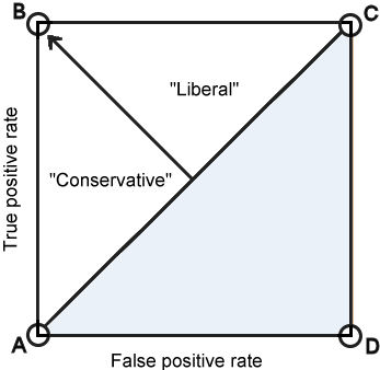
• Point A (0, 0) is a classifier that never identifies any case as positive - no false positive errors, but all positive cases are false-negative errors.
• Point C (1, 1), is the converse. All cases are labelled as positives and there are now no false-negative errors.
• Point B (0, 1) is the ideal classifier with perfect classification.
• Point D (1, 0) is a strange classifier which labels every case incorrectly. Inverting the predictions creates a perfect classifier.
• The diagonal line from the A to C represents chance performance, tossing a coin would give same accuracy. Any classifier in the grey area below this line is performing worst than chance.
• Any classifier whose performance is the upper left triangle is doing better than chance. Better classifiers are towards the point of the arrow (top left).
• Classifiers close to the A-C line can be tested to determine if their performance is significantly better than chance.
• Classifiers to the left of the arrow are "conservative", i.e. they make positive classifications only with strong evidence. This produces few false positive errors, but it tends to misclassify many positive cases as negative.
• Classifiers to the right of the arrow are "liberal", i.e. they make positive classifications with weak evidence. This means that they tend to get positive cases correct but at the expense of a high false positive rate.

Try the self assessment question (opens in a new window).

ROC curves

If a classifier does not provide the continuous values needed for a ROC plot only a single confusion matrix is possible. This produces a ROC plot with a single point. However, if raw scores are available thresholds can be adjusted to produce a series of points the form the ROC curve.

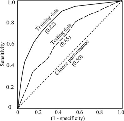
A ROC curve is obtained by plotting all sensitivity values (true + fraction) on the y axis against their equivalent (1 - specificity) values (false + fraction) for all available thresholds on the x axis. The quality of the approximation to a curve depends on the number of thresholds tested. If a small number are tested the 'curve' will resemble a staircase.

The area under the ROC curve (AUC) is an index of performance that is independent of any particular threshold (Deleo, 1993). AUC values are between 0.5 and 1.0, with 0.5 indicating that the scores for two groups do not differ, while a score of 1.0 indicates no overlap in the distributions of the group scores. An AUC of 0.75 indicates that, for 75% of the time, a random selection from the positive group will have a score greater than a random selection from the negative class.

A ROC plot does not provide a rule for the classification of cases. However, there are strategies that can be used to develop decision rules from the ROC plot which depend on having values for the relative costs of false + and false - errors. As a guideline Zweig and Campbell (1993) suggest that if the false + costs (FPC) exceed the false - costs (FNC) the threshold should favour specificity, while sensitivity should be favoured if the reverse is true. Combining these costs with the prevalence (p) of positive cases allows the calculation of a slope (Zweig and Campbell, 1993).

m = (FPC/FNC) x ((1-p)/p)

m is the slope of a tangent to the ROC plot. The point at which this tangent touches the curve identifies the particular sensitivity/specificity pair that should be used to select the threshold. If costs are equal FNC/FPC = 1, and m is the ratio of negative to positive cases with a slope of 1 for equal proportions. As the prevalence declines m becomes increasingly steep.

top

---

Costs

All binary classifiers share two potential mistakes. If they are equivalent the optimal rule is to assign a case to the class that has highest posterior probability, given the predictors. Typically, this will be the largest class. If the mistakes are not equivalent they should be weighted by attaching costs. Despite the apparent subjectivity of costs there are many situations in which there is an obvious inequality. For example, in a cancer screening programme the cost of a false negative error far exceeds that of a false positive. It is less clear what the relative costs should be, the only certainty is that it should not be 1:1.

Few biological studies explicitly include costs in the classifier design and evaluation. However, all studies implicitly apply costs because a failure to explicitly allocate costs results in the default, and least desirable, equal cost model. Unfortunately, it is impossible to provide advice on specific values for misclassification costs because these will always involve subject-specific judgements.

Types of cost

Turney (2000) recognised nine levels of cost in classifier design and use. First are the misclassification of cases, broken down into five sub-categories.

• constant cost (a global, but different, cost for each class);
• case-specific costs that vary between cases (for example if a class was "extinction prone" the cost could take account of the population size for each species);
• case-specific costs that depend on a value for a predictor rather than the class;
• time-sensitive costs, conditional on the timing of the misclassification;
• costs that are conditional on other errors.

Other costs relate to the development of the classifier and include costs related to obtaining the data and the computational complexity.

Using misclassification costs

Misclassification cost are relatively easily represented in a two-class predictor. The aim changes from one of minimising the number of errors (maximising accuracy) to one which minimises the cost of the errors. Consequently, the imposition of costs complicates how the classifier's performance is assessed. There are different methods by which costs can be applied.

• Vary the allocation threshold so that misclassification costs are optimised.
• Weight cases or oversample to make the most cost-sensitive class the majority class. In general, classifiers are more accurate with the majority class.
• Most common method is a cost matrix that weights errors prior to the accuracy calculation. For example, in a conservation-based model costs could be assigned as weights that take account of perceived threats to the species. The cost associated with an error depends upon the relationship between the actual and allocated classes. Misclassification costs need not be reciprocal, for example classifying A as B may be more costly than classifying B as A. Lynn et al. (1995) used a matrix of misclassification costs to evaluate the performance of a decision-tree model for the prediction of landscape levels of potential forest vegetation. Their cost structure was based on the amount of compositional similarity between pairs of groups
.

top

---

Resources