
Intended Learning Outcomes
At the end of this section students should be able to complete the following tasks.
- Describe the structure of a generalised additive model.
- Explain why GAMS are said to be semi-parametric.
- Explain how the form of the smoothing function affects the analysis.
Background
Generalized additive models (GAM) are semi-parametric extensions of the generalised linear model. They are partially parametric because the probability distribution of the class variable must be specified. Typically, in a classifier, the class variable would normally be from the binomial distribution. However, they are not fully parametric because the link function is a 'smoothed' relationship, with a form that is determined by the data rather than some pre- defined theoretical relationship.
In a GAM the usual coefficients or weights are replaced by non-parametric relationships, modelled by smoothing functions, resulting in a model with the form g(L) = si(xi), a more general form of the generalized linear model. The si(xi) are the smoothed functions.
The main advantage of GAMs is that they can deal with highly non-linear and non-monotonic relationships between the class and the predictors without the need for the explicit use of variable transformations or polynomial terms. This is because the GAM smoothing functions do these tasks automatically. In this respect the smoothing functions are similar to the hidden layer in an artificial neural network.
Although they have some advantages over GLMs they are more complicated to fit and may be difficult to interpret.
Smoothing functions
Smoothing functions produce line, with a user-defined complexity, to describe the general relationship between a pair of variables, in this case the class and a predictor. Loess and lowess smoothers are locally weighted regression analyses that find arbitrarily complex (non- parametric) relationships between two variables. Unlike the usual regression methods they build up a series of local neighbourhoods rather than estimating a global relationship. They differ in the order of the local regression with loess using a quadratic, or second degree, polynomial and lowess a linear polynomial.
If a neighbourhood or span is established around a particular case it is possible to fit a local regression line to this neigbourhood. Normally, the span is specified as a percentage of the data points, e.g. a span of 0.50 uses half of the points. These neighbouring points are weighted by their distance from the central case (x), with weights becoming smaller as data points become more distant from x. All cases outside the span have zero weight and hence no effect on the local fit. Because local lines are fitted to each data point, and then merged, it is possible for the lines to have very different slopes depending on the local trend. The size of the span affects the complexity of the smoothed relationship, with larger spans giving smoother fits. A span that is too small will produce a 'spiky' line that models the error in the data. Conversely, spans that are too wide will miss important local trends. Useful values of the smoothing parameter typically lie in the range 0.25 to 0.75.
The example below is a scatterplot of the length and breadth (mm) of raven eggs from the Highland
region of Scotland (the data are from the Derek Ratcliffe's (1993) The Peregrine Falcon 2nd
edition. Four levels of smoothing were used (0.2 - red line, 0.4 - blue line, 0.6 - hashed black line
and 0.8 - solid black line). As the level of smoothing increases the line becomes simpler and a close
approximation to a straight line.
Example data
This example uses the same data that were analysed in the first logistic
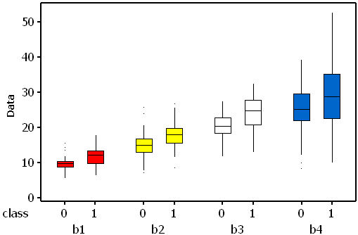
regression analysis. The data are available as an Excel file or a plain text file. There are four continuous predictors (b1 to b4) and two
classes with 75 cases per class. Class means differ significantly for all predictors.
This implies that all four predictors should be useful to identify the class of a case.
Three of the predictors (b1-b3) are uncorrelated with each other (p < 0.05
for all pair-wise correlations). Predictors b3 and b4 are highly correlated (r = 0.7),
but b4 is not correlated with b1 or b2. In all predictors the mean for class 1 is larger than that for class
0.If effect sizes (difference in the means divided by the standard deviation) are
calculated it is possible to estimate the expected rank order for the standardised weights. In data set B
the expected order is (b1 = b3), b2 and b4.
Analysis preliminaries
These analyses were carried out using the gam function from R. The default smoothing algorithm, used by this function, is a B-spline smoother. It is important to apply a constraint so that the smoothed B-splined curve does not become too 'wiggly'. As with narrow spans, a curve that is too complex will end up modelling the noise in the data rather than the overall trend. If the smoothed line is too complex it is likely that the analysis will generate false optimism about future performance on new data. Conversely, a line that is too simple, for example a straight line, would fail to capture any non-linearity in the relationship and it is likely to produce a poor classifier. A compromise is achieved by incorporating a penalty term. In the R implementation the degree of smoothness is controlled indirectly by specifying the effective degrees of freedom, which is used to adjust the penalty term. Four degrees of freedom is equivalent to a third degree polynomial.
Because the degree of smoothing is one of the most important parameters in the GAM analysis four analyses are described. The first two use the default B-spline smoother with four and one degrees of freedom. Four degrees of freedom is probabaly too large (may be fitting nosie) for these data while one is too few (linear model). These values were selected so that they should over-, and under-, fit the data respectively. The other two analyses use loess smoothers with spans of 0.25 and 0.75 respectively. Again, the smaller span should overfit the data while the other may be a better alternative. The analyses will be compared with each other and with the logistic regression of the same data.
Analysis 1 B-Spline smoothers and AIC
The residual deviances for the two analyses were 98.5 (133.0 df) for the analysis using 4 df and 121.1 (145.0 df) for the analysis with 1 df. The Null deviance, i.e. before any model is fitted, is 207.9 (149 df) for these data. This means that the changes in deviance have been 109.4 (207.9 - 98.5) and 86.8 (207.9 - 121.1) respectively. In a logistic regression analysis SPSS calls this change the model chi-square and it is used to test a hypothesis that the predictors have improved the model by reducing the amount of unexplained variation. Note that the model deviance in the logistic regression analysis was 121.3, which is almost identical to the model with the simpler smoother. This is not too surprising since the use of 1 df has forced the analysis to model linear relationships between the class and the predictors. The larger decrease in the deviance, with the more complex fit, is to be expected but it is important to:
- Question if the improvement is 'worth' the lost of more error df (139 comared with 145).
- Question if the model which uses the more complex smoother will perform better with novel data, or has the gain been obtained at the cost of a loss of generality (i.e. the model has fitted too much of the noise)?
Both models have four predictors but the extra smoothing of the more complex model uses up degrees of freedom. This effect can be incorporated into the calculation of the AIC (Akaike's Information Criterion), which can be used to judge the relative merits of the models. The AIC can be found from (-2(LL) + 2k), where -2LL is the residual deviance and k is number of parameters that are estimated during the model's development. k is not the number of predictors, since it must also include all of the terms used in the smoothers. k is, therefore, the difference between the number of cases and the model residual degrees of freedom. For example, in the first model, with 4 df, the residual df are 133. Since there are 150 cases, k = 150 - 133 = 17. Therefore, AIC is 98.5 + 2 x 17 = 132.5. In the second model AIC = 121.1 + (2 x (150-145)) = 131.3. The inclusion of 2k in the AIC calculation penalizes the addition of extra parameters (e.g. more complex smoothers or additional predictors). The AIC is used to select or rank models, the best being the one which has a good fit but with the minimum number of parameters, i.e the samllest AIC. There is little to choose between these two models, based on their raw AIC scores. However, Delta AICs (AIC - minimum AIC) are preferred to raw AIC values because they force the best, of the tested models, to have a Delta AIC of zero and thereby allow meaningful comparisons without the scaling issues that affect the AIC (Burnham and Anderson 2004 (pdf file)). The Delta AIC values for the more complex model is 1.2, suggesting that there is little to separate these models. However, in the spirit of parsimony the simpler model would be better. But, extending the principle of parsimony, there is little benefit in using a GAM for these data since its performance is almost identical to that of the equivalent logistic regression. Burnham and Anderson (2004) provide much more information about the AIC, and the related BIC (Bayesian Information Criterion), in their online conference paper.
The significance of the predictors, as judged by their non-parametric Chi-squared values, are shown in the table below.
| 4 df | 1 df | |||||
|---|---|---|---|---|---|---|
| Predictor | df | ChiSq | p | df | ChiSq | p | B1 | 3 | 4.204 | 0.240 | 0 | 0.007 | 0.019 | B2 | 3 | 6.738 | 0.081 | 0 | 0.046 | 0.019 | B3 | 3 | 11.845 | 0.008 | 0 | 0.078 | 0.006 | B4 | 3 | 2.602 | 0.457 | 0 | 0.068 | 0.023 |
Only B3 is significant when 4 df were used for the B-spline function. Recall that this will fit more complex lines than the straight lines obtained using 1 df. In the second analysis all four preditors are significant. In the equivalent logistic regression only b4 was insignificant. The following partial plots show the modelled relationships between the class and the predictors. The two models (1 and 4 df) are shown side by side. Note the linear relationship for the 1 df models
| Predictor | 1 df B-spline | 4 df B-spline |
|---|---|---|
| B1 |  |
 |
| B2 |  |
 |
| B3 |  |
 |
| B4 |  |
 |
Analysis 2 Loess smoothers
The residual deviances for the two analyses were 62.3 (116.0 df) for the analysis using the 0.25 span and 122.9 (138.1 df) for the analysis with 0.75. This means that the changes in deviance were 145.6 (207.9 - 62.3) and 85.0 (207.9 - 122.9) respectively. The AIC values are (62.3 + 2 x 34) 130.3 and (121.9 + 2 x 11.9) 145.7 respectively, giving a Delta AIC of 15.4. Burnham and Anderson (2004) suggest that such a large Delta AIC means that there is little support for the model using the 0.75 span.
| 0.75 span | 0.25 span | |||||
|---|---|---|---|---|---|---|
| Predictor | df | ChiSq | p | df | ChiSq | p | B1 | 1.6 | 1.802 | 0.321 | 7.7 | 21.773 | 0.004 | B2 | 2.1 | 5.331 | 0.076 | 7.9 | 17.501 | 0.024 | B3 | 1.3 | 9.323 | 0.004 | 5.9 | 15.183 | 0.018 | B4 | 1.9 | 0.898 | 0.605 | 7.5 | 21.477 | 0.004 |
As in the previous analyses only B3 is significant when the wider span was used. Recall that this will fit less complex lines than those obtained using a narrower span. Again, in the second analysis, all four preditors are significant. In the equivalent logistic regression only b4 was insignificant. The following partial plots show the modelled relationships between the class and the predictors. The two models (0.75 and 0.25 spans) are shown side by side. Note the complex relationships for the smaller span.
| Predictor | 0.75 span | 0.25 span |
|---|---|---|
| B1 |  |
 |
| B2 |  |
 |
| B3 |  |
 |
| B4 |  |
 |
Comparing the models
There are two ways in which these four models, plus the equivalent logistic regression, can be compared. The first looks at their predictive accuracy based on the area under the ROC curve (AUC).
| GAM Model | AUC | 95% LCL | 95% UCL |
|---|---|---|---|
| loess 0.75 span | 0.910 | 0.865 | 0.956 |
| loess 0.25 span | 0.967 | 0.838 | 0.995 |
| B-spline 1 df | 0.896 | 0.847 | 0.945 |
| B-spline 4 df | 0.923 | 0.880 | 0.965 |
The model with a loess smoother, and a 0.25 span, has the largest AUC. The value of 0.967 suggests that it makes very few prediction errors, indeed using re-substituted values only four class 1 and twelve class 0 cases are missclassified (see below). The AUC for the B-spline model with 1 df is identical to that achieved by the logistic regression.
However, is this accuracy only possible because the gam model is over-fitting the training data and would, therefore, perform poorly with new data? This aspect is the focus of the next self-assessment exercise.
The second comparison uses the model AIC and Delta AIC values.
| Model | AIC | Delta AIC |
|---|---|---|
| B-spline 1 df | 131.3 | 1.0 |
| B-spline 4 df | 132.5 | 2.2 |
| Loess 0.75 span | 145.7 | 15.4 |
| Loess 0.25 span | 130.3 | 0.0 |
| Logistic regression | 131.3 | 1.0 |
Although there is little to choose between three of the models, the best the GAM model uses the loess smoother with a 0.25 span. This was also the best with respect to the AUC values. However, the AIC for the logistic regression is only slightly larger, perhaps suggesting that this is the better alternative. It is interesting that the AIC for the logistic regression is identical to that for the GAM with the simplest B-spline smoother (1 df). As a further test two of the GAM models are tested with novel data. This is because the modelled relationships look quite complex and the best GAM model may not do well in more robust tests (see the next self-assessment exercise).